An Introduction to Maximum Likelihood Estimation

In statistics, maximum likelihood estimation (MLE) is a fundamental technique used to estimate the parameters of a probability distribution based on observed data. The mathematical formulation of MLE can be intimidating if you haven’t seen it before, but the idea motivating it is extremely simple and has deep connections to abductive reasoning, also known as inference to the best explanation. Here, I go over the basics of MLE as the first part in a series of posts explaining the connection between it and least squares regression. To begin, let’s informally discuss a concrete example and then we’ll try to generalize what we learn from it and get more rigorous.

Note: in this post I use MLE to refer both to the technique of maximum likelihood estimation, but also to the estimate itself

Flipping Biased Coins

Imagine you are given a biased coin (a coin for which the odds of flipping heads or tails is not $50/50$) and are tasked with approximating the probability with which it lands heads. You have nothing at your disposal, no way to directly measure the weightedness of the coin. All you can do is flip it and see the outcome. How do you go about doing this? Your intuition probably tells you to observe a bunch of coin flips and simply count the frequency of heads. Our gut tells us that for a sufficiently high number of flips this number should approach the true probability. But is there a way to reason our way there without relying purely on intuition? Let’s try.

Firstly, since we know there are only two possible outcomes we can say that if $P(H) = \theta$ then it must be the case that $P(T) = 1 - \theta$. Additionally, we know that we have to observe a large number of flips before we can say much of anything about the probabilities, and we also know that these flips are all independent of one another. Let’s call the number of flips we observe $n$. Finally, if you’ve been exposed to basic probability theory you might remember that the probability of two independent events co-occuring is the product of their individual probabilities. To convince yourself of this, consider the case of flipping two fair coins. The probability of observing any one pair is $\frac{1}{4}=\left(\frac{1}{2}\right)^2$ because we have $4$ distinct outcomes, $2$ for each coin A1. $P(H, T) = P(H)P(T)$ With this information we can write the probability of observing a particular set of $n$ coin flips which we denote as $\mathcal{D}$ given a particular probability of flipping heads $\theta$: $P(\mathcal{D} \mid \theta) = \overbrace{\theta \cdot \theta \cdots \theta\cdot\theta}^{\mathclap{\text{times we flip heads}}} \cdot \underbrace{(1 - \theta)(1 - \theta)\cdots(1 - \theta)(1 - \theta)}_{\mathclap{\text{times we flip tails}}} =\theta^k(1 - \theta)^{n - k}$ where $k$ is the number of times we flip heads and $n - k$ is the number of times we flip tails.

Now, ask yourself the following question: given some observed set of flips $\mathcal{D}$, what value for $\theta$ maximizes $P(\mathcal{D})$; what value of $\theta$ makes our observed dataset most probable? Said another way, given a set of flip outcomes, what value for $P(H)$ could we choose that would maximize the chances of observing those outcomes? That number is the maximum likelihood estimate. $\hat{\theta}_{\text{MLE}}=\argmax_\theta{P(\mathcal{D}\mid \theta)}$ At first encounter the MLE estimate can often feel slippery or circular. We are using our data to approximate a model that best explains…our data. However, MLE is really the operationalization of a deep intuition: given an outcome, what conditions would have most likely led to that outcome? The mathematical formulation may not be as intuitive, but the underlying idea is beautifully straightforward.

"At a superficial level, the idea of maximum likelihood must be prehistoric: early hunters and gatherers may not have used the words 'method of maximum likelihood' to describe their choice of where and how to hunt and gather, but it is hard to believe they would have been surprised if their method had been described in those terms."₁

If we have some data, and we are willing to assume that it comes from a particular distribution (a normal distribution, for example), along with some other things, then MLE finds what parameters to give that distribution to make it most consistent with our data. In this example we arrived at our distribution through reasoning about the flipping process, and now we are trying to find the value for its parameter $\theta$ which will best explain our data.

Okay, lets see MLE in action. We are tasked with solving the following optimization problem $\argmax_{\theta}P(\mathcal{D}\mid\theta) = \argmax_{\theta}\left[\theta^k(1 - \theta)^{n - k}\right]$ The solution to said problem will be our estimate $\hat{\theta}_{\text{MLE}} \approx \theta$ which is the approximate probability of our biased coin flipping heads. To start we can notice that whatever argument maximizes our function will also maximize its logarithm. This is because the logarithm is a monotonically increasing function. Reframing the problem this way will allow us to get rid of those annoying exponents and turn multiplication into addition A2. $\begin{aligned} \argmax_{\theta}\left[\theta^k(1 - \theta)^{n - k}\right] &= \argmax_{\theta}\left[\log(\theta^k(1 - \theta)^{n - k})\right] \\ &= \argmax_{\theta}\left[\log(\theta^k) + \log((1-\theta)^{n-k})\right]\\ &= \argmax_{\theta}\left[k\log\theta + (n-k)\log(1-\theta)\right] \end{aligned}$ So far all we have done is some algebraic manipulation of $P(\mathcal{D} \mid \theta)$. Now to solve the optimization problem, we can take the derivative of our function and solve for its maximum by setting that equal to zero. $\begin{aligned} \frac{d}{d\theta}\log P(\mathcal{D}\mid\theta) &= \frac{d}{d\theta}\left[k\log\theta + (n-k)\log(1-\theta)\right]\\ &=\frac{k}{\theta} - \frac{n-k}{1-\theta} \end{aligned}$ Now we set our equation equal to $0$, replace $\theta$ with $\hat{\theta}_{\text{MLE}}$, and solve. For succinctness I will write $\hat{\theta}_{\text{MLE}}$ as $\hat{\theta}$ $\begin{aligned} 0 &= \frac{k}{\hat{\theta}} - \frac{n-k}{1-\hat{\theta}}\\ &=\frac{k(1-\hat{\theta})\hat{\theta}}{\hat{\theta}} - \frac{(n-k)(1-\hat{\theta})\hat{\theta}}{1-\hat{\theta}}\\ &= k(1 - \hat{\theta}) - \hat{\theta}(n - k)\\ &= k - k\hat{\theta} - n\hat{\theta} + k\hat{\theta} \\ &= k - n\hat{\theta}\\ \hat{\theta}_{\text{MLE}} &= \frac{k}{n} \end{aligned}$ And so at the end of all of that we find that the maximum likelihood estimate for the probability of flipping heads given a dataset is simply the frequency of head occurences in our data. Our intuitions have been confirmed! That was a lot of math for such a simple answer, but granted this was a pretty simple problem. Can the MLE generalize to a larger problem space where it’s harder for our intuition to guide us? The answer is yes, but before we get there, lets simulate some coin flips and see how our estimate does as the size of our dataset increases.

import matplotlib.pyplot as plt
import numpy as np
# Parameters
true_theta = 0.65   # True theta
n_flips = 1000  # Number of coin flips
trials = 50   # 50 trials of 1000 flips each
trial_outcomes = []
for trial in range(trials):
    # Simulate coin flips
    outcomes = np.random.binomial(n=1, p=true_theta, size=n_flips)  # 1 is heads, 0 is tails
    mle = np.cumsum(outcomes) / np.arange(1, n_flips + 1)
    trial_outcomes.append(mle)
# Plotting
for i, outcome in enumerate(trial_outcomes):
    if i == 0:
        plt.plot(outcome, label=r'$\frac{k}{n}$', lw=0.6)
    else:
        plt.plot(outcome, lw=0.6)
plt.axhline(y=true_theta, color='black', linestyle='--', label='True Probability of Heads')
plt.title('50 Estimates of P(H)')
plt.xlabel('Number of Coin Flips')
plt.ylabel('Cumulative Probability of Heads')
plt.legend()
plt.tight_layout()
plt.show()

Figure 1. The maximum likelihood estimate computed for 50 trials with $n=1000$ and $P(H)=0.65$

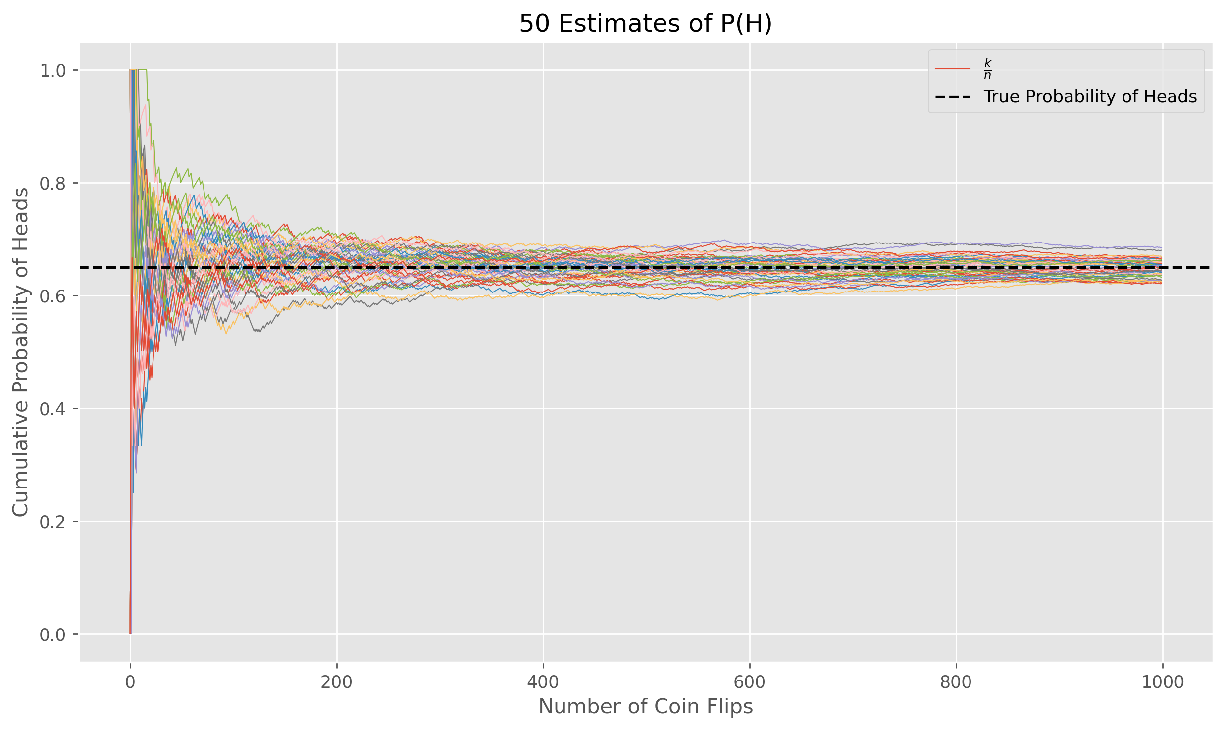
In the image above, I plot the evolution of $50$ estimates of $P(H)$ as more coin flip landings are observed and used to update the MLE. Qualitatively we can tell our intuition that “more data is better” was also correct. As $n$ gets larger we see our estimates getting closer to the true value, albeit with most of the progress happening within the first $400$ observations. In fact, although we won’t prove it here, under some basic assumptions it can be shown that in the limit, as our number of data points approaches infinity, the MLE estimate actually converges to the true value of $\theta$.

Generalizing the MLE

One of the most compelling attributes of maximum likelihood estimation is its broad applicability. MLE is not limited to specific distributions or data types; it can be applied to any situation where a likelihood function can be constructed. However, in its simplest formulation (the one discussed in this post) there are some strong assumptions we have to make about our data for the technique to work well. In the remainder of this post I will go over MLE in its general formulation and highlight what those assumptions are.

We begin by observing a set of data points $X_1, X_2, \dots, X_n$ which are assumed to be independent and identical samples from a probability distribution $P(X; \theta)$, where $X$ represents the domain of the distribution and $\theta$ represents its parameters. We don’t know the value(s) of $\theta$ (that’s the point of MLE) but we know the class of distributions (normal, Poisson, etc.) to which $P$ belongs. Ultimately what we want from MLE is a data informed approximation of $\theta$ which we refer to as $\hat{\theta}_{\text{MLE}}$. Using this estimate we will be able to paramaterize a distribution which reflects our observations and which allows us to make statistical propositions about our dataset.

The first step in MLE is to construct a likelihood function $\mathcal{L}(\theta)$ $\mathcal{L}_n(\theta) = \prod_{i=1}^n P(X_i; \theta)$ The above equation says that our likelihood function $\mathcal{L}(\theta)$ is the cumulative product (A3) of our probability distribution $P$ evaluated at each of our data points $X_i$ for a given parameterization $\theta$. The fact that the likelihood is a function over the parameters and not the data is important to note and implicit in this equation is all of the assumptions needed for MLE:

(1) Our data is comprised of independent, uncorrelated samples (hence the cumulative product)
(2) Each data point was sampled identically ($P$ is unchanging across data points)
(3) We know the form of $P$, though obviously not the exact values of $\theta$

But what does the likelihood function actually tell us? The likelihood function serves as a bridge between our data and our possible choices for parameters. It is a function that quantifies the ability of a particular estimate of $\theta$ to explain our data. If we were to choose a value for $\theta$ and plug it in to $\mathcal{L}(\theta)$ we would get a number quantifying the plausibility of that $\theta$ given the observed data. Note that previously we were using the notation $P(\mathcal{D}\mid\theta)$, but this is really the same idea. For a given value of $\theta$ what is the probability of our data?

To make this point more clear, let’s go back to the coin example. If we were to flip our coin $10$ times and observe that it landed on heads $8$ out of those $10$, what would be the shape of $\mathcal{L}(\theta)$? The function now looks like $\mathcal{L}(\theta) = \theta^8(1-\theta)^2 \qquad 0 \leq \theta \leq 1$ What does this look like plotted?

def likelihood_function(n_heads: int, n_tails: int, theta: float) -> float:
    return (theta ** n_heads) * ((1 - theta) ** n_tails)
theta_values = np.linspace(0, 1, 1000)
heads, tails = 8, 2
plt.plot((likelihood_function(heads, tails, theta_values)))
plt.xticks(np.arange(0, 1001, 100), [f'{0.1 * i:0.2f}' for i in range(11)])
plt.xlabel(r'$\theta$')
plt.ylabel(r'$\mathcal{L}(\theta)$')
plt.legend()
plt.show()

Figure 2. $\mathcal{L}(\theta)$ when $k=8, n=10$

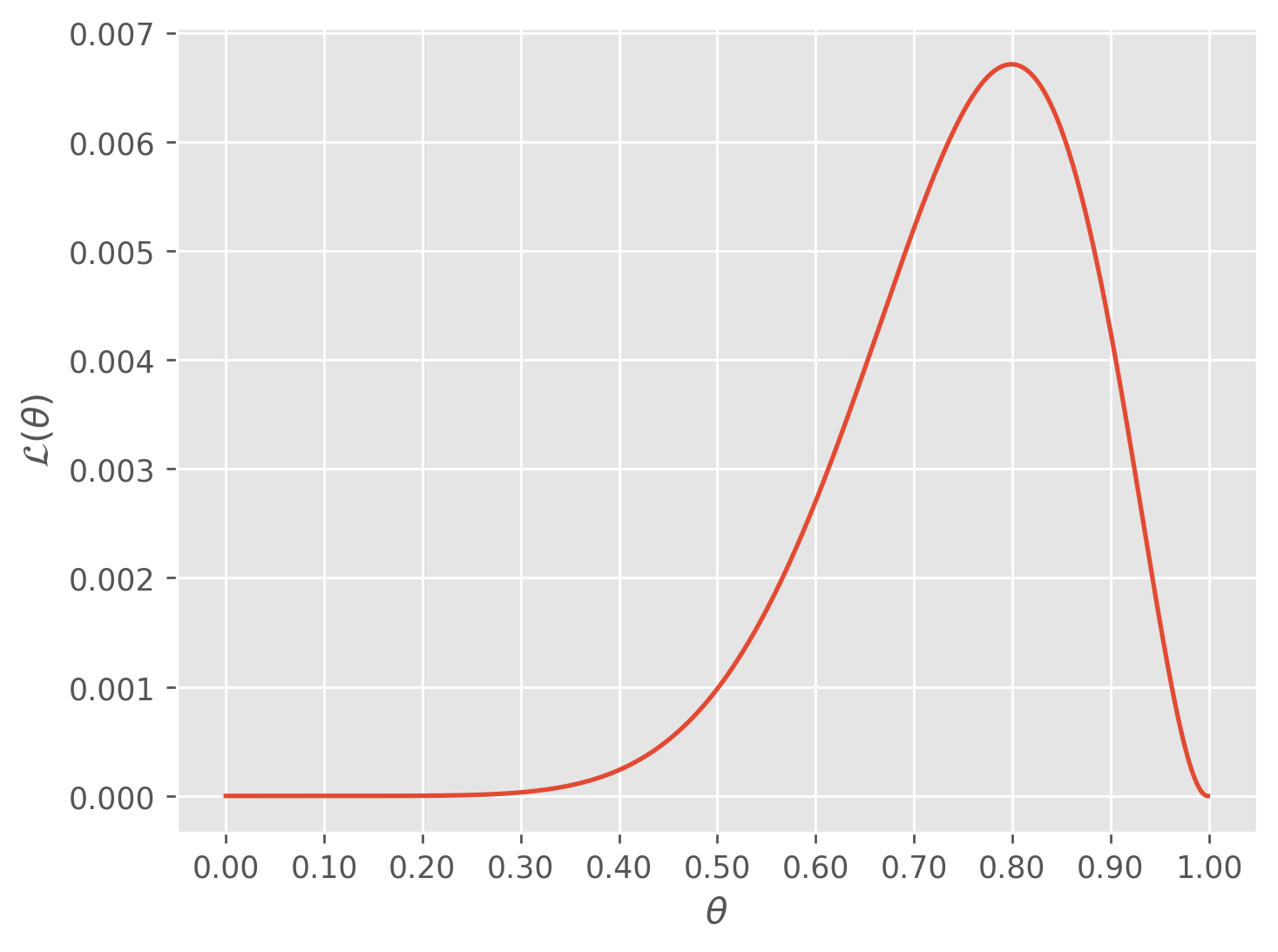
As you can see, our function is clearly maximized at $\theta=0.8$ exactly as expected from our work in the previous section. This is the big point of MLE. If we were to choose any value but $\frac{k}{n}$ for $\theta$, $\mathcal{L}(\theta)$ which is the probability of our data under different choices of $\theta$, would be smaller. Thus given the data $(k=8,\enspace n-k=2)$ the probability of observing our data is maximized when we choose $\theta=\hat{\theta}_{\text{MLE}}=0.8$

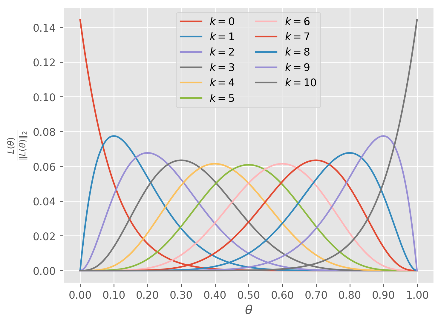
What would $\mathcal{L}(\theta)$ look like for a different set of observations? If we were to have some other frequency of heads, the curve above would swing between $1$ and $0$ but would always have a maximum value at $\frac{k}{n}$

theta_values = np.linspace(0, 1, 1000)
heads = np.arange(11)
for n_heads in heads:
    n_tails = 10 - n_heads
    likelihood = likelihood_function(n_heads, n_tails, theta_values)
    plt.plot(likelihood / np.linalg.norm(likelihood), label=fr'$k = {n_heads}$')
plt.xticks(np.arange(0, 1001, 100), [f'{0.1 * i:0.2f}' for i in range(11)])
plt.xlabel(r'$\theta$')
plt.ylabel(r'$\frac{L(\theta)}{\Vert L(\theta)\Vert_2}$')
plt.legend(ncol=2)
plt.show()

Figure 3. Diagram of the likelihood function as we sweep over values of $k$ and keep $n$ fixed at $10$. The function has been normalized here for visualization purposes. In reality, for $k\neq 0, k\neq 10$, the heights are much smaller.

So now if we understand that the likelihood function allows us to put a value for $\theta$ in and get a measure of its ability to explain our data out, it follows that if we want to find an approximation for the true $\theta$ we should choose the $\theta$ which maximizes the likelihood function.

Let’s now continue with our generalized version of MLE.

The raw likelihood function is $\mathcal{L}_n(\theta)=\prod_{i=1}^nP(X_i; \theta)$. In general, products are more difficult to work with than sums, both analytically and numerically, and so in practice we always work with the log-likelihood function $L(\theta)$. $L_n(\theta) = \log{\mathcal{L}_n(\theta)} = \log\prod_{i=1}^n P(X_i; \theta) = \sum_{i=1}^n \log{P(X_i; \theta)}$ As was noted before, transforming the likelihood function like this does not change the $\theta$ which maximizes the function. Now, all that’s left to do is find the $\argmax$ over $\theta$. Typically this involves taking the derivative of $L_n(\theta)$ and finding the global maximum by solving for the value of $\theta$ that makes that equal $0$. $\begin{aligned} \hat{\theta}_{\text{MLE}} &= \argmax_{\theta}{L_n(\theta)}\\ &= \theta \enspace \text{st} \enspace \frac{d}{d\theta}L_n(\theta) = 0 \end{aligned}$ Depending on the specifics of the particular likelihood function this may be difficult to do analytically.

A Final Example

As a final example let’s find the maximum likelihood estimate for the Poisson distribution which has parameter $\lambda$. The Poisson distribution expresses the probability of a given number of events happening in a fixed interval of time or space, and is given by $P(X; \lambda) = \frac{\lambda^X e^{-\lambda}}{X!}$ where $k$ is the number of events and $\lambda$ is the mean rate of occurences in the interval. $\begin{aligned} \mathcal{L}_n(\lambda) &= \prod_{i=1}^n \frac{\lambda^{x_i} e^{-\lambda}}{x_i!}\\ L_n(\lambda) = \log(\mathcal{L}_n(\lambda)) &=\log\left[\prod_{i=1}^n \frac{\lambda^{x_i} e^{-\lambda}}{x_i!}\right]\\ &=\sum_{i=1}^n\log\left({\frac{\lambda^{x_i} e^{-\lambda}}{x_i!}}\right)\\ &=\sum_{i=1}^n\log{\lambda^{x_i}} + \log{e^{-\lambda}} - \log{x_i!}\\ &=\sum_{i=1}^nx_i\log\lambda -\lambda - \log x_i!\\ L_n(\lambda)&=-n\lambda + \sum_{i=1}^nx_i\log{\lambda} - \log{x_i!}\\ \frac{d}{d\lambda}L_n(\lambda)&=-n + \frac{\sum_{i=1}^nx_i}{\lambda}\\ 0 &= -n + \frac{\sum_{i=1}^nx_i}{\hat{\lambda}_{\text{MLE}}}\\ \hat{\lambda}_{\text{MLE}} &= \frac{1}{n}\sum_{i=1}^nx_i \end{aligned}$ Thus, the maximum likelihood estimator for the Poisson distribution is simply the sample mean.

Appendix

A1
If this seems unintuitive to you, imagine you have a pair of unweighted $6$-sided die and want to know the probability of rolling a $6$ with both of them. If you were to roll a $1$ first, you haven’t effected the outcome of the second roll and so there are still $6$ possible outcomes. The key is to realize that this is actually true no matter what number we roll first and so for each outcome of the first roll we have $6$ possible outcomes for the second. Thus our total number of possibilities is $6 \cdot 6 = 36$ and so the probability of any one outcome is $\frac{1}{36}$. In fact, if we had $3$ die then we would have $6^3$ possibilities each with probability $\frac{1}{6^3}$. Or if we added a coin flip we would have $2 \cdot 6^2$ possibilities each with probability $\frac{1}{72}$ because for each of the $36$ outcomes from the die rolling we could flip either heads or tails. All of this is a function of the events being independent from one another, and would not work if the outcomes of one process altered the outcomes of another.

A2
The logarithm of a product is the sum of the logarithms of the products factors $\log{xy} = \log{x} + \log{y}$ Notice that this necessitates $\log{x^n} = n\log{x}$ A3
If you aren’t familiar with this notation, capital pi $\Pi$ is used to denote the cumulative product of a sequence. $\prod_{i=1}^n x_i = x_1 \cdot x_2 \cdots x_{n-1} \cdot x_n$ This is exactly what we did for the flipped coin example, where we wrote the likelihood as the cumulative product of the probability of each flip. In that example there were only two possible probabilities and so there was no need for this notation, we could just use exponents.