Building a Spike Sorter

In neuroscience, we often work with electrophysiology recordings for which the number of neurons recorded is unknown. This is due to the fact that most recordings are extracellular, meaning we don’t insert the microelectrode directly into a cell, but instead insert it into the interstice between neighboring cells where voltage fluctuations from any nearby neurons can influence the recorded signal. The reason for this is the difficulty of intracellular insertion and the stability of the recording thereafter. This begs the question: how then do we disambiguate between different neurons in our recording? This problem is referred to as spike sorting and there exists many decades of algorithmic and probabalistic approaches to solving it (a classic review).

State of the art algorithms take advantage of high channel density electrodes in which the same neuron can be “heard” on multiple channels simultaneously, allowing for more sophisticated techniques which utilize information from these multiple sources. In this post, I aim to implement a much more simple algorithm for spike sorting $1$-dimensional recordings, with the hope that for what we give up in relevance to the cutting edge we will gain back in intuition, learning, and practicability.

Note: this post was made in part as a reading for [a class I designed for UW] NEUSCI 490 and so its pacing and scope differ form the usual posts I make.

Designing our algorithm

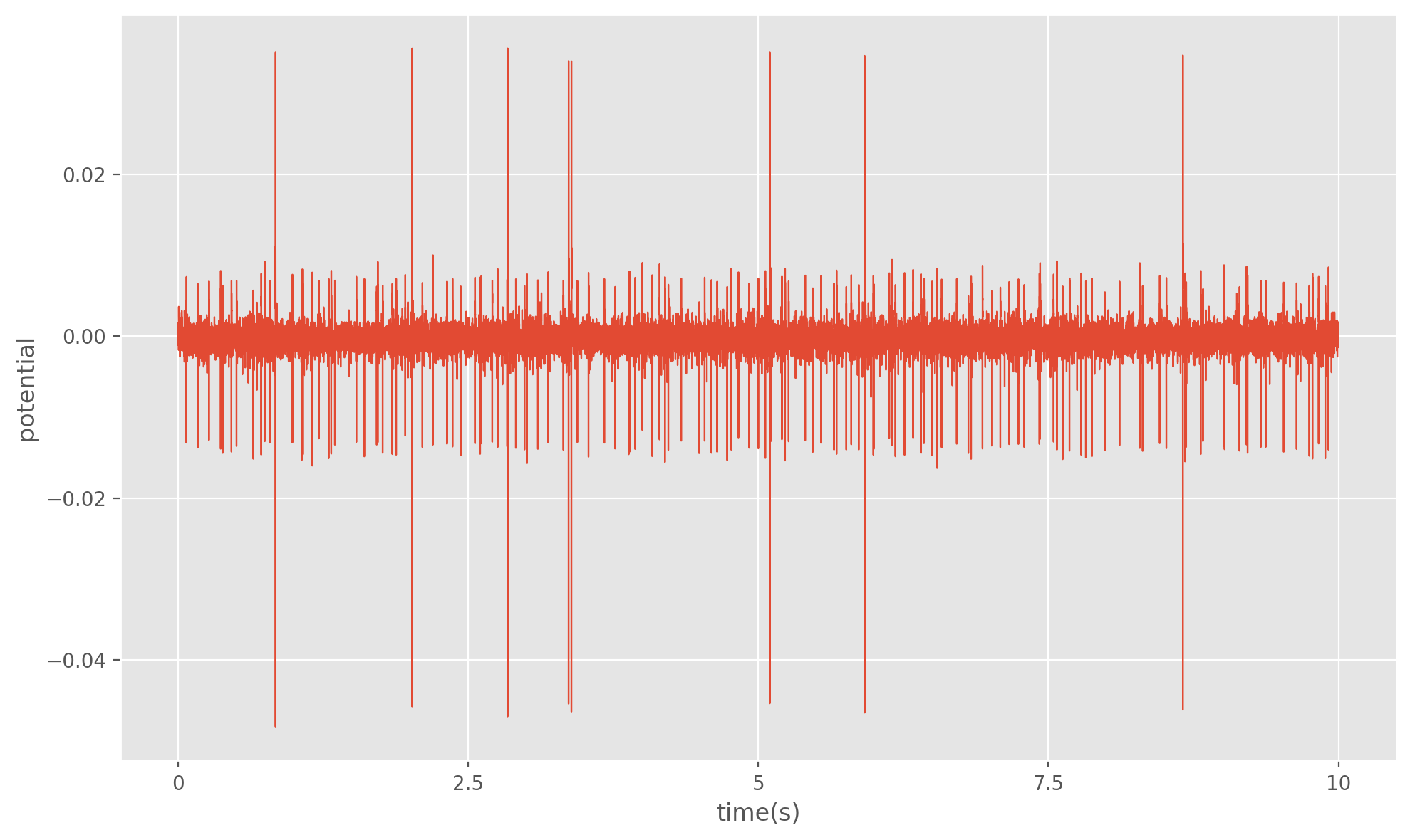
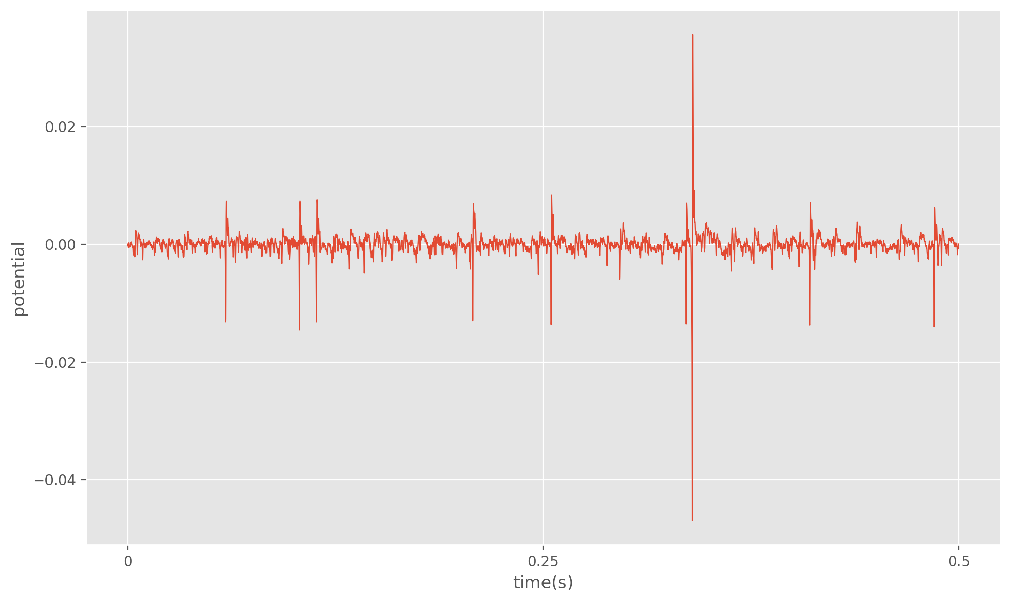
To begin designing our algorithm, let’s state the problem more formally. Suppose we are given a $1$-dimensional recording of a voltage signal $V(t)$. We can model this signal as the sum of the voltage contribution $s(t)$ from $K$ different neurons around the recording location, plus a “noise” term $\varepsilon(t)$ A1. $V(t) = \sum_{i=1}^K s_i(t) + \varepsilon(t)$ For an interval of time in our recording we can expect to see a spike from any of the $K$ neurons with some probability. Thus the problem of spike sorting not only involves determining the number of signal sources $K$, but also determing the spike times for each of our $K$ sources. Here a spike is defined as a rapid rise and fall in voltage that exceeds a predefined threshold. For our implementation we will determine our spike times first, and then use the shape of $V(t)$ in some window around those spike times (referred to as the spike waveform) to determine the number of neurons. Some angles of leverage we typically have over our data is that spike amplitude and waveforms can vary quite a lot between neurons within a recording. It is also worth noting that an individual neurons contribution to $V$ when it is not spiking is typically impossible to distinguish from $\varepsilon$. For most analyses however, the spike times and/or waveforms are our ultimate goal and so this is not a problem.

Figure 1. An extracellular recording in which at least two neurons are clearly present.

The procedure for our algorithm will be as follows.

1. Preprocess our signal
2. Detect spikes and extract waveforms
3. Reduce the dimensionality of our waveforms
4. Cluster waveform representations

Preprocessing

Often times in electrophysiology data there exists low frequency components (typically $< 300\text{Hz}$) in the recorded signal that do not reflect the faster transients of spikes. Activity in these low frequency bands are interesting in their own right, but for our purposes they are an additional source of complexity we would like to get rid of. To do this we will utilize filtering to remove certain frequencies from our signal. To understand filtering we will need to take a quick detour to familiarize ourselves with Fourier analysis.

Fourier analysis, a quick aside

Fourier analysis is a field of mathematics that deals with extracting periodic components from signals. The field encompasses many techniques that are key to signal processing and neuroscience. At the foundation of Fourier analysis is the concept of a Fourier series, which says that any periodic signal can be decomposed into an infinite sum of trigonometric functions at different amplitudes and frequencies. This means that something as rigid and non-smooth as a step-function/square wave, can be expressed by just adding up many many $\sin$ and $\cos$ functions A2.

Figure 1. A square wave and its Fourier approximations to the first few terms.

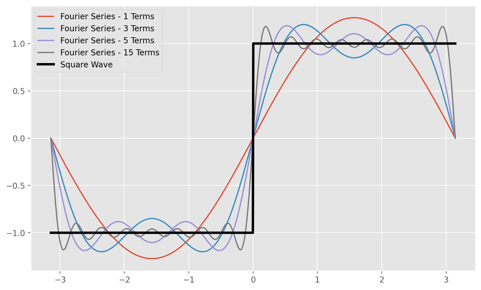
How we determine those amplitudes and frequencies is beyond the scope of this post and would require a few lectures from a signals and systems course, however we can still apply Fourier analysis to manipulate our data. If you want some intuition for why Fourier series work, you can think about how sin waves which are out of phase with one another deconstructively interfere to cancel out. Now imagine you have infinite sin waves of varying frequencies and amplitudes, Fourier analysis says that there exists a certain unique combination of frequencies and amplitudes for which the interference between all the component waves results in any periodic function we would like. If we extend Fourier series to non-periodic functions the technique is called the Fourier transform which is a ubiquitous and powerful technique in applied mathematics. This means that any non-periodic function, even our recording $V(t)$ can be decomposed into its contributing frequencies. Thus, if

Spike Detection and Waveform Extraction

Waveform Processing

Waveform Clustering

Appendix

A1
The use of scare quotes here is to signal that beyond electrical noise we are dealing with essentially deterministic processes. If we had perfect information about the kinetics of every single particle around the electrode we wouldn’t think of their influence on $V$ as “noise”.

A2
Code for building Fourier series plot

import numpy as np
import matplotlib.pyplot as plt
def square_wave(x):
    return np.sign(np.sin(x))

def fourier_term(n, x):
    if n % 2 == 0:
        return 0  # Fourier series for square wave includes only odd terms
    return (4 / (np.pi * n)) * np.sin(n * x)

def fourier_series(N, x):
    return sum(fourier_term(n, x) for n in range(1, N + 1))

# Plotting
x = np.linspace(-np.pi, np.pi, 1000)
y = np.linspace(-np.pi, np.pi, 1000)
N_terms = [1, 3, 5, 15]  # Different numbers of terms in the Fourier series
plt.figure(figsize=(10, 6))
for N in N_terms:
    plt.plot(x, fourier_series(N, x), label=f'Fourier Series - {N} Terms')
plt.plot(x, square_wave(x), label='Square Wave', color='black', linewidth=3)
plt.grid(True)
plt.legend()
plt.show()