K-Means and Gaussian Mixture Models

In machine learning, clustering encompasses a family of problems and techniques for grouping unlabeled data into categories. In contrast to classification, where our job is to learn relationships between data and their associated labels, in clustering our job is to learn the labels themselves by leveraging the patterns and structure present in the data. To make this more concrete, imagine you are given two datasets containing images of cats and dogs. The datasets are identical except that in the first dataset each image comes with a label cat or dog, and in the second you only are given the image. In classification our job is to learn what features of the image are most predictive of the label (cat ears, dog nose, etc.), whereas in clustering our job is to learn how to group similar images together without any pre-existing labels. That is, to identify clusters that correspond to cat and dog based solely on the inherent features and patterns observed in the images.

The vast majority of data is unlabeled, yet the need for effective algorithmic techniques to extract meaningful information from such data is critical for its use. From the grouping of genetic sequences to identify disease patterns, to image segmentation, uses for clustering abound. In this post I introduce the problem of clustering and derive two popular techniques: $K$-means and Gaussian mixture models (GMM). To begin I will apply $K$-means to the Old Faithful dataset to give a concrete example of clustering before using the techniques shortcomings to motivate GMMs.

$K$-Means

The $K$-means algorithm is a simple and intuitive approach to clustering that doesn’t require any probability theory to understand. Suppose we are given some data set $\mathcal{D}$ consisting of $N$ Euclidean vectors. $\mathcal{D} = \{\mathbf{x}_1 \dots \mathbf{x}_n \dots \mathbf{x}_N\}$ In our example dataset each vector is $2$-dimensional, but $K$-means still works in higher dimensions. Importantly, we have no other additional information. Unlike classification, we have no class labels to work with, only the raw coordinates of each data point.

Figure 1. The normalized old faithful dataset. In the unmodified data the axes represent the duration of an eruption and the time till the next eruption for the Old Faithful geyser in Yellowstone National Park.

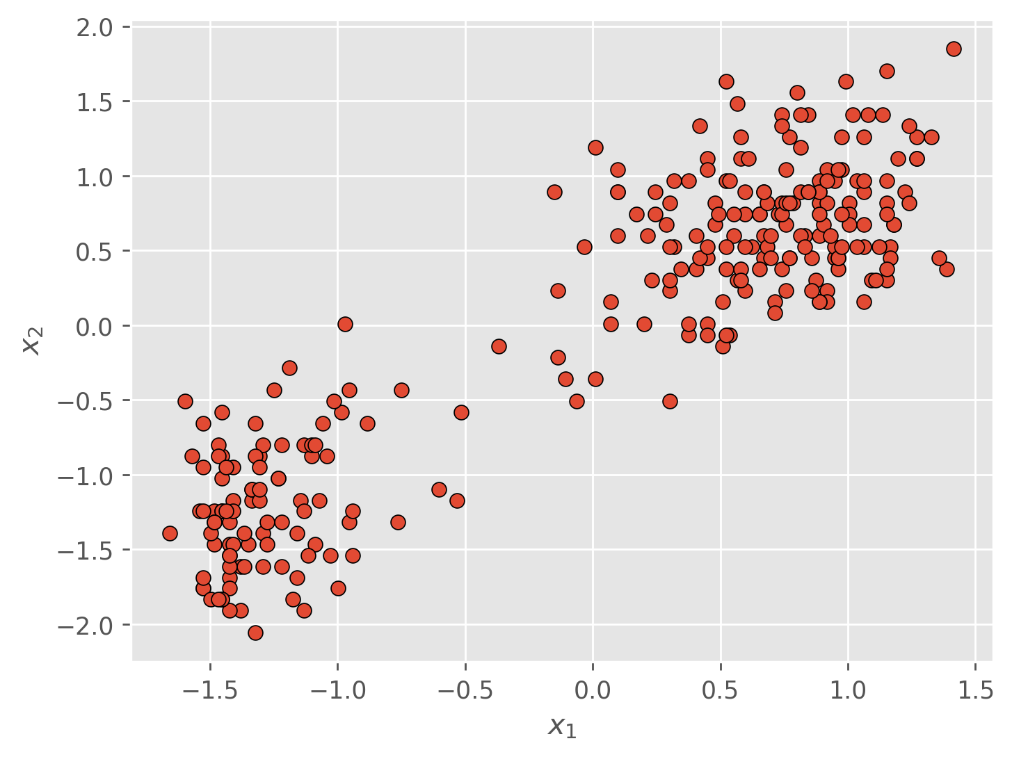
We would like to partition the dataset above into $K$ sub-groups such that each data point $\mathbf{x}_n$ is associated with a unique cluster $k$. Intuitively, we would like similar data points to be clustered together and dissimilar data points to be clustered apart. It just so happens that in our dataset it is visually obvious how we should assign points to clusters, but in practice our data is rarely this nice. Our goal is essentially to categorize or classify this unlabeled data. In doing so we will depart from classification and optimize not just the boundary of the clusters, but the labels associated with each data point as well.

To begin, we’ll introduce two variables. The first is a set of $K$ vectors $\{\boldsymbol{\mu}_1, \dots, \boldsymbol{\mu}_K\}$ where $\boldsymbol{\mu}_k$ is the centroid or prototype of the $k^{th}$ cluster. You can think of $\boldsymbol{\mu}_k$ as the center of mass for cluster $k$. We will also introduce an indicator variable $z_{n,k}$ where $z_{n,k} = 1$ if the $n^{th}$ data point belongs to cluster $k$ and $0$ otherwise. Our goal then, is to optimize our set of cluster centroids $\{\boldsymbol{\mu}_k\}$ and our cluster assignments $z_{n, k}$ such that the sum of the squared distances from each data point to its assigned centroid is minimized. In plain language, if we are going to assign a point to a particular cluster, we would like the center of that cluster to be as close as possible to the point. We can write out this objective with the following equation $J = \sum_{n = 1}^N\sum_{k = 1}^Kz_{n, k}\Vert\mathbf{x}_n - \boldsymbol{\mu}_k\Vert^2_2$ Our job then is to choose the values for $z_{n, k}$ and $\boldsymbol{\mu}_k$ that minimize $J$ $\argmin_{r_{n, k}, \boldsymbol{\mu}_{k}}\sum_{n = 1}^N\sum_{k = 1}^Kz_{n, k}\Vert\mathbf{x}_n - \boldsymbol{\mu}_k\Vert^2_2$

Finding $z_{n, k}$

Intuitively, the value for $z_{n, k}$ that minimizes $J$ is simply the one which assigns its associated data point to the closest cluster center. More formally $z_{n, k} = \begin{cases} 1 & \text{if } k = \argmin_j \Vert \mathbf{x}_n - \boldsymbol{\mu}_j \Vert^2_2 \\ 0 & \text{otherwise} \end{cases}$

Finding $\boldsymbol{\mu}_k$

To find the values for $\boldsymbol{\mu}_k$ that minimize $J$ we’ll start by taking its derivative with respect to $\boldsymbol{\mu}_k$ $\begin{aligned} \frac{\partial J}{\partial \boldsymbol{\mu}_k} &= \frac{\partial}{\partial\boldsymbol{\mu}_k}\sum_{n = 1}^N\sum_{k = 1}^Kz_{n, k}\Vert\mathbf{x}_n - \boldsymbol{\mu}_k\Vert^2_2\\ &= \frac{\partial}{\partial\boldsymbol{\mu}_k}\sum_{n=1}^N z_{n, k}\Vert\mathbf{x}_n - \boldsymbol{\mu}_k\Vert^2_2\\ &= \frac{\partial}{\partial\boldsymbol{\mu}_k}\sum_{n=1}^N z_{n, k}(\mathbf{x}_n - \boldsymbol{\mu}_k)^\top(\mathbf{x}_n - \boldsymbol{\mu}_k)\\ &= -2\sum_{n=1}^N z_{n, k}(\mathbf{x}_n - \boldsymbol{\mu}_k) \end{aligned}$ Now we can set the derivative equal to $0$ and solve for $\boldsymbol{\mu}_k$ $\begin{aligned} 0 &= -2\sum_{n=1}^N z_{n, k}(\mathbf{x}_n - \boldsymbol{\mu}_k) \\ &= \sum_{n=1}^N z_{n, k}\mathbf{x}_n - z_{n, k}\boldsymbol{\mu}_k \\ \sum_{n=1}^N z_{n, k}\boldsymbol{\mu}_k &= \sum_{n=1}^N z_{n, k}\mathbf{x}_n \\ \boldsymbol{\mu}_k \sum_{n=1}^N z_{n, k} &= \sum_{n=1}^N z_{n, k}\mathbf{x}_n \\ \boldsymbol{\mu}_k &= \frac{\sum_{n=1}^N z_{n, k}\mathbf{x}_n}{\sum_{n=1}^N z_{n, k}} \end{aligned}$ The denominator in the above equation is the number of data points assigned to the $k^{th}$ cluster, and so $\boldsymbol{\mu}_k$ is simply the average of its assigned points.

Now notice that the equations for our two parameters each contains the other parameter as a variable. This motivates an iterative, algorithmic solution in which we optimize one parameter while fixing the other, and then optimize the second parameter holding the first one fixed. Our procedure will go like this:

$K$-means Algorithm

(1) Initialize our cluster centers $\boldsymbol{\mu}_k$
(2) Compute our assignments $z_{n, k}$ with our current value for $\boldsymbol{\mu}_k$
(3) Using our new assignments, compute new cluster centers $\boldsymbol{\mu}_k$
(4) Repeats steps (2) and (3) until changes in $J$ between steps are negligible.
Implementation

Figure 2. Iterations of the $K$-means algorithm on the rescaled Old Faithful data set

Figure 3. $K$-means objective function during fitting.

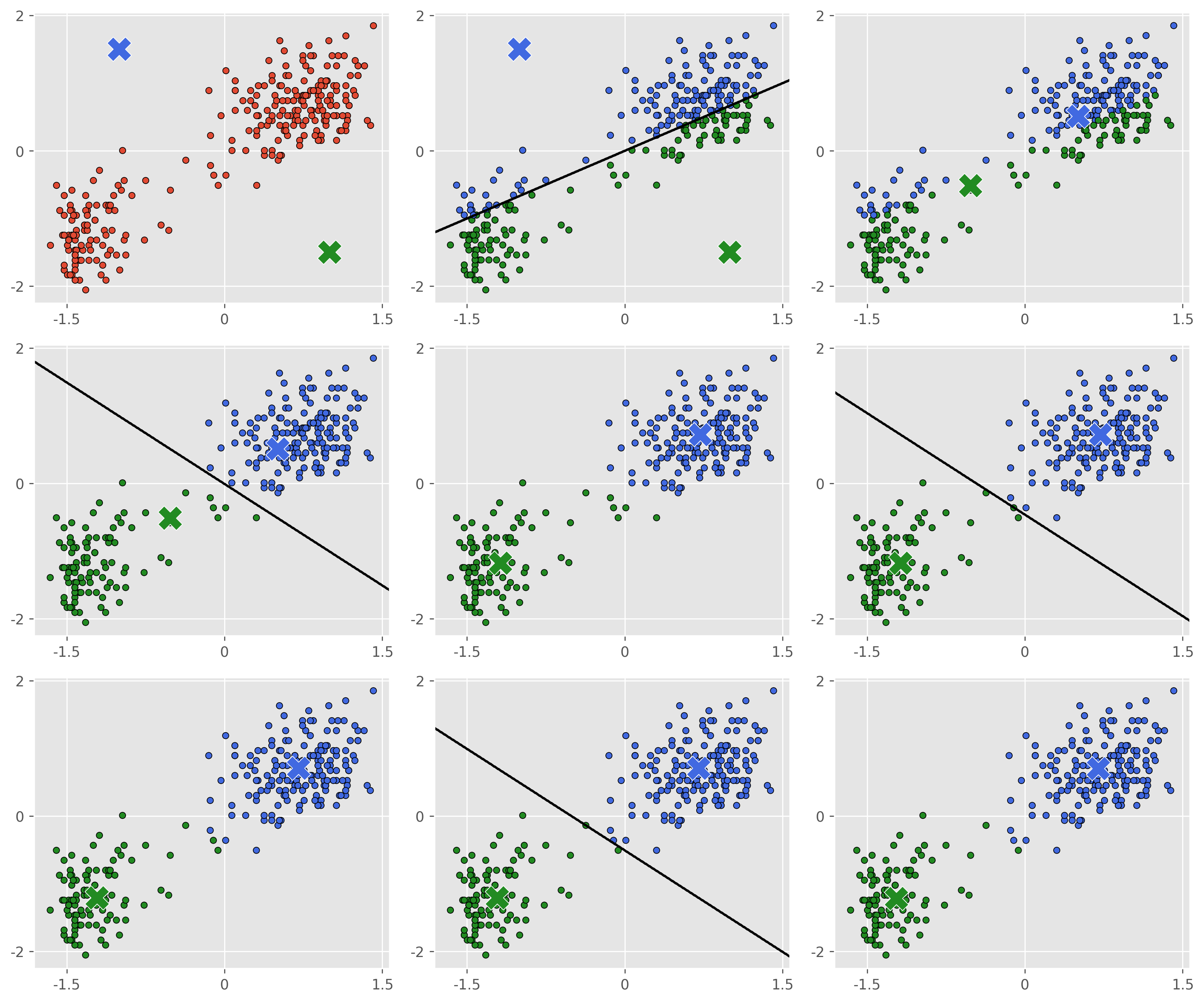
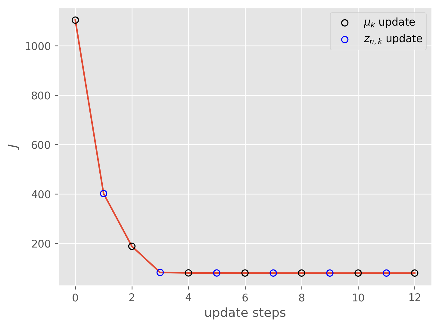
As you can see, for this dataset the algorithm converges extremely quickly and we get a decent clustering in only a few optimization steps. In practice $K$-means is often a good first choice for clustering, but the technique does have some serious drawbacks.

Perhaps the most obvious drawback is that we have no principled way of choosing the number of clusters $K$. In fact a larger number of clusters will always result in a lower value of $J$. In our toy example this isn’t a problem, largely because our data is 2-dimensional and so we can visualize it, but if our data were to be higher dimensional than this would be more difficult. There does exist some metrics for determining the optimal cluster number, but these have their flaws as well. In addition, $K$-means can be quite sensitive to the initialization of $\{\boldsymbol{\mu}_k\}$, particularly when our data is not as easily separable as our toy example. There does exist initialization strategies which help to alleviate this, but there are more problems. One is that our objective function $J$ models our clusters as equally sized spheres, an assumption which will not hold in many (maybe most) circumstances. Finally, $K$-means gives us back hard cluster assignments, when sometimes we’d like to have a confidence or probability that a data point belongs to a particular cluster.

Luckily, our next technique will allow us to address almost all of these shortcomings.

Gaussian Mixture Model

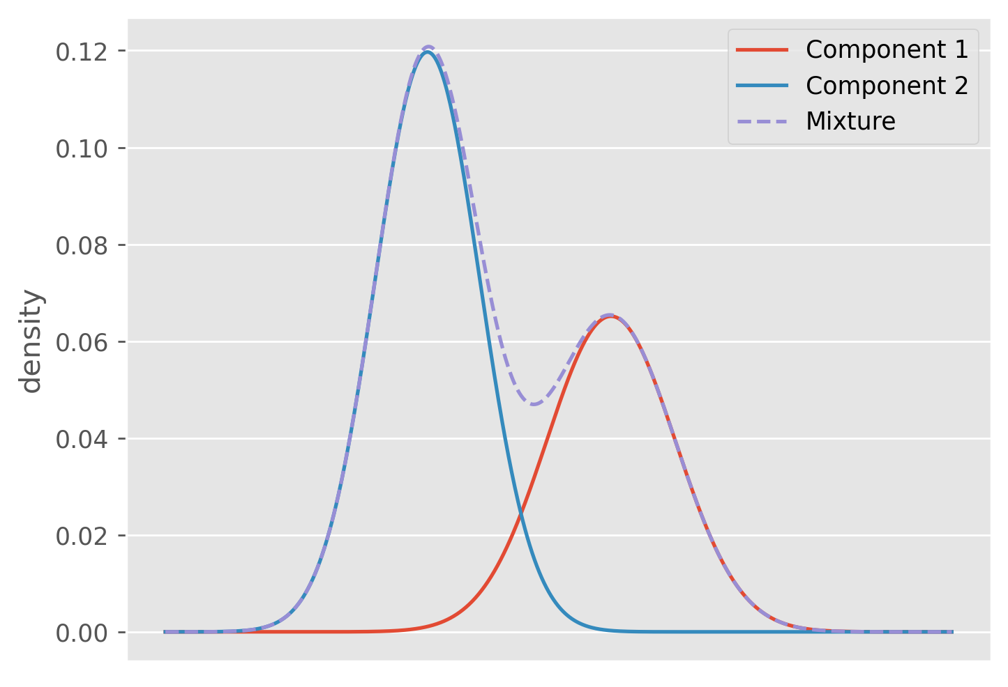
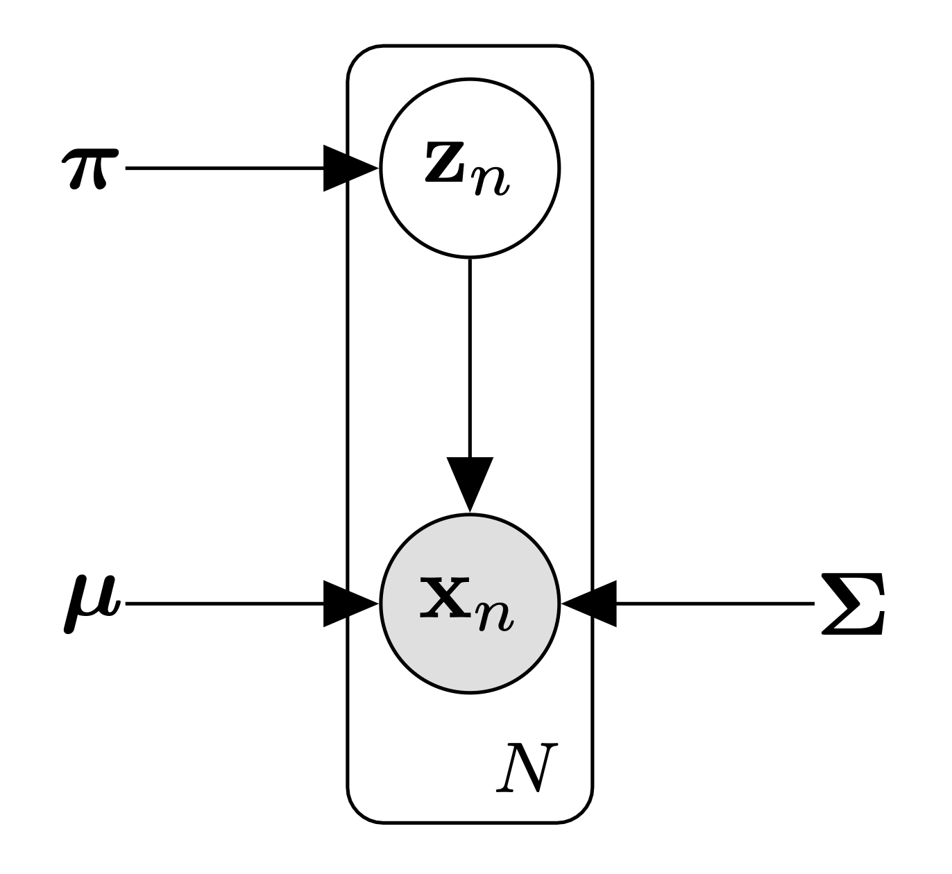Gaussian mixture models (GMM) are a powerful probabilistic tool for solving the clustering problem that will help to ameliorate many of the problems we faced with $K$-means. A GMM is a just a linear combination of $K$ Gaussian distributions where each component is weighted by some scalar $\pi_k$ such that $\sum_{k=1}^K\pi_k = 1$. This constraint allows us to interpret the combination itself as a probability distribution. We will interpret each Gaussian component as the distribution of a particular cluster. For any one data point $\mathbf{x}$ the GMM says it has a probability given by $p(\mathbf{x}) = \sum_{k=1}^K \pi_k \cdot \mathcal{N}(\mathbf{x}\mid \boldsymbol{\mu}_k, \bold{\Sigma}_k)$ Where $\boldsymbol{\mu}_k$ and $\bold{\Sigma}_k$ are the mean and covariance of the $k^{th}$ component respectively.

Figure 4. Example GMM with two components

To start we will introduce a set of variables $z_n$ just like we did with $K$-means, where $z_n \in \{1, \dots, K\}$ indicates the cluster identity for the $n^{th}$ data point. Constructing a set of unobserved variables like this is extremely common in unsupervised learning problems. Often times we refer to these $z$ variables as latent variables. We said before that we interpret our mixture components as our clusters, and so we have $p(z = k) = \pi_k$ This just means that the probability a data point comes from cluster $k$ is equal to its weighting in the mixture. We can also write out the distribution of $\mathbf{x}$ conditioned on the value of $z$. $p(\mathbf{x} \mid z=k) = \mathcal{N}(\mathbf{x}\mid \boldsymbol{\mu}_k, \bold{\Sigma}_k)$ This is just the distribution of the $k^{th}$ cluster.

To fit this model to our data we will rely on maximum likelihood estimation (MLE) which I wrote about in my previous post. MLE will allow us to determine the optimal values for our model parameters $\bold{\Theta} = \{\pi_k, \boldsymbol{\mu}_k, \bold{\Sigma}_k\}$. To start we first must construct our likelihood function $p(\{\mathbf{x}\}\mid \bold{\Theta}) = \prod_{n=1}^N p(\mathbf{x}_n)$ Because of how we formulated our latent variables we can rewrite $p(\mathbf{x}_n)$ as a marginal of the joint distribution between $z$ and $\mathbf{x}$. $\begin{aligned} \prod_{n=1}^N p(\mathbf{x}_n) &= \prod_{n=1}^N \sum_{k=1}^K p(\mathbf{x}_n, z=k) \\ &= \prod_{n=1}^N\sum_{k=1}^K p(z=k)p(\mathbf{x}_n\mid z=k) \\ &= \prod_{n=1}^N\sum_{k=1}^K \pi_k \cdot \mathcal{N}(\mathbf{x}_n\mid \boldsymbol{\mu}_k, \bold{\Sigma}_k) \end{aligned}$ Now we can take the log of this expression to get our log-likelihood $\mathcal{L} = \log p(\{\mathbf{x}\}\mid \bold{\Theta}) = \sum_{n=1}^N \log \left[ \sum_{k=1}^K \pi_k \cdot \mathcal{N}(\mathbf{x}_n\mid \boldsymbol{\mu}_k, \bold{\Sigma}_k)\right]$ The MLE procedure now tells us to find the values for $\{\pi_k\}, \{\boldsymbol{\mu}_k\}$ and $\{\bold{\Sigma}_k\}$ that maximize $\mathcal{L}$. First let’s find the maximum likelihood estimate for $\boldsymbol{\mu}_k$.

Finding $\boldsymbol{\mu}_k$

We’ll start by taking the derivative of $\mathcal{L}$ with respect to $\boldsymbol{\mu}_k$ $\begin{aligned} \frac{\partial\mathcal{L}}{\partial\boldsymbol{\mu}_k} &= \frac{\partial}{\partial\boldsymbol{\mu}_k}\sum_{n=1}^N \log \left[ \sum_{k=1}^K \pi_k \cdot \mathcal{N}(\mathbf{x}_n\mid \boldsymbol{\mu}_k, \bold{\Sigma}_k)\right]\\ &=\sum_{n=1}^N \frac{\partial}{\partial\boldsymbol{\mu}_k} \log \left[ \sum_{k=1}^K \pi_k \cdot \mathcal{N}(\mathbf{x}_n\mid \boldsymbol{\mu}_k, \bold{\Sigma}_k)\right] \end{aligned}$ Here we can apply the chain rule A2 $\begin{aligned} \frac{\partial\mathcal{L}}{\partial\boldsymbol{\mu}_k} &= \sum_{n=1}^N \frac{\frac{\partial}{\partial\boldsymbol{\mu}_k} \Bigl(\sum_{k=1}^K\pi_k\cdot\mathcal{N}(\mathbf{x}_n \mid \boldsymbol{\mu}_k, \bold{\Sigma}_k)\Bigr)} {\sum_{k=1}^K\pi_k\cdot\mathcal{N}(\mathbf{x}_n \mid \boldsymbol{\mu}_k, \bold{\Sigma}_k)} \\ &=\sum_{n=1}^N\frac{\pi_k\cdot\mathcal{N}(\mathbf{x}_n \mid \boldsymbol{\mu}_k, \bold{\Sigma}_k)\cdot\bold{\Sigma}_k^{-1}(\mathbf{x}_n - \boldsymbol{\mu}_k)} {\sum_{j=1}^K\pi_j\cdot\mathcal{N}(\mathbf{x}_n \mid \boldsymbol{\mu}_j, \bold{\Sigma}_j)} \end{aligned}$ Refer to A3 for that last step.

Now to clean things up a bit let’s define a new parameter $\gamma_{n, k}$ which we will define as $\gamma_{n, k} = \frac{\pi_k\cdot\mathcal{N}(\mathbf{x}_n \mid \boldsymbol{\mu}_k, \bold{\Sigma}_k)}{\sum_{j=1}^K\pi_j\cdot\mathcal{N}(\mathbf{x}_n \mid \boldsymbol{\mu}_j, \bold{\Sigma}_j)}$ This quantity will appear a lot going forward and abstracting it this way will help us notationally, however this term also has a rich meaning: it is the conditional probability of $z$ given $\mathbf{x}$. To see this we can use Bayes Rule $\begin{aligned} p(z_n = k \mid \mathbf{x}_n) &= \frac{p(z_n = k)p(\mathbf{x}_n \mid z_n=k)}{\sum_{j=1}^K p(z_n = j)p(\mathbf{x}_n \mid z_n = j)}\\ &=\frac{\pi_k\cdot\mathcal{N}(\mathbf{x}_n \mid \boldsymbol{\mu}_k, \bold{\Sigma}_k)}{\sum_{j=1}^K\pi_j\cdot\mathcal{N}(\mathbf{x}_n \mid \boldsymbol{\mu}_j, \bold{\Sigma}_j)} \\ &=\gamma_{n, k} \end{aligned}$ This understanding allows us to view $\pi_k$ as the prior probability that $z_n = k$ before observing $\mathbf{x}_n$, and $\gamma_{n, k}$ as the posterior probability that $z_n = k$ after we observe $\mathbf{x}_n$. $\gamma_{n, k}$ is also often referred to as the responsibility because it can be viewed as the ability of the $k^{th}$ cluster to explain the value of $\mathbf{x}_n$. Also, notice that $\sum_{k=1}^K \gamma_{n, k} = 1$. This should make sense because in our model each data point has to come from a cluster.

Now we can plug $\gamma_{n, k}$ into our derivative and set it equal to $0$ to solve for $\boldsymbol{\mu}_k$ $\begin{aligned} 0 &= \sum_{n=1}^N \gamma_{n, k} \bold{\Sigma}_k^{-1}(\mathbf{x}_n - \boldsymbol{\mu}_k)\\ &=\bold{\Sigma}_k^{-1} \sum_{n=1}^N \gamma_{n, k}\mathbf{x}_n - \gamma_{n, k}\boldsymbol{\mu}_k\\ \sum_{n=1}^N \gamma_{n, k}\boldsymbol{\mu}_k &= \sum_{n=1}^N \gamma_{n, k}\mathbf{x}_n\\ \boldsymbol{\mu}_k &= \frac{\sum_{n=1}^N \gamma_{n, k}\mathbf{x}_n}{\sum_{n=1}^N \gamma_{n, k}}\\ \boldsymbol{\mu}_k &= \frac{\sum_{n=1}^N \gamma_{n, k}\mathbf{x}_n}{N_k}\\ \end{aligned}$ So after all of that, we have this nice result that the center of cluster $k$ is a weighted average of the data where the weights are the responsibilities or the ability of that cluster to explain the data. The denominator is the sum of the responsibility of the $k^{th}$ cluster across every data point, and so you can think about it almost like the effective number of data points assigned to cluster $k$.

I will leave derivations of the maximum likelihood estimates for $\pi_k$ and $\bold{\Sigma}_k$ in the appendix, but they too have nice interpretations. $\bold{\Sigma}_k = \frac{1}{N_k}\sum_{n=1}^N\gamma_{n, k}(\mathbf{x}_n - \boldsymbol{\mu}_k)(\mathbf{x}_n - \boldsymbol{\mu}_k)^\top\qquad \pi_k = \frac{N_k}{N}$ Like $\boldsymbol{\mu}_k$, our covariance estimate is a weighted empirical covariance of the data where the weights are the responsibilities of the $k^{th}$ cluster, whilst $\pi_k$ is the effective fraction of the data assigned to cluster $k$.

Notice that, as was the case in $K$-means, our values for $\gamma_{n, k}$ are dependent on our parameters, whilst our parameters are themselves dependent on $\gamma_{n, k}$. Like with $K$-means, this motivates an iterative approach in which we alternate between computing the responsibilities and optimizing the parameters. The procedure will go like this:

GMM Algorithm

(1) Initialize our parameters $\boldsymbol{\mu}_k, \bold{\Sigma}_k, \pi_k$
(2) Compute responsibilities $\gamma_{n, k}$
(3) Using our new responsibilities, update out parameters
(4) Repeats steps (2) and (3) until changes in $\mathcal{L}$ between steps are negligible.
Implementation

Figure 2. Iterations of our GMM fitting procedure.

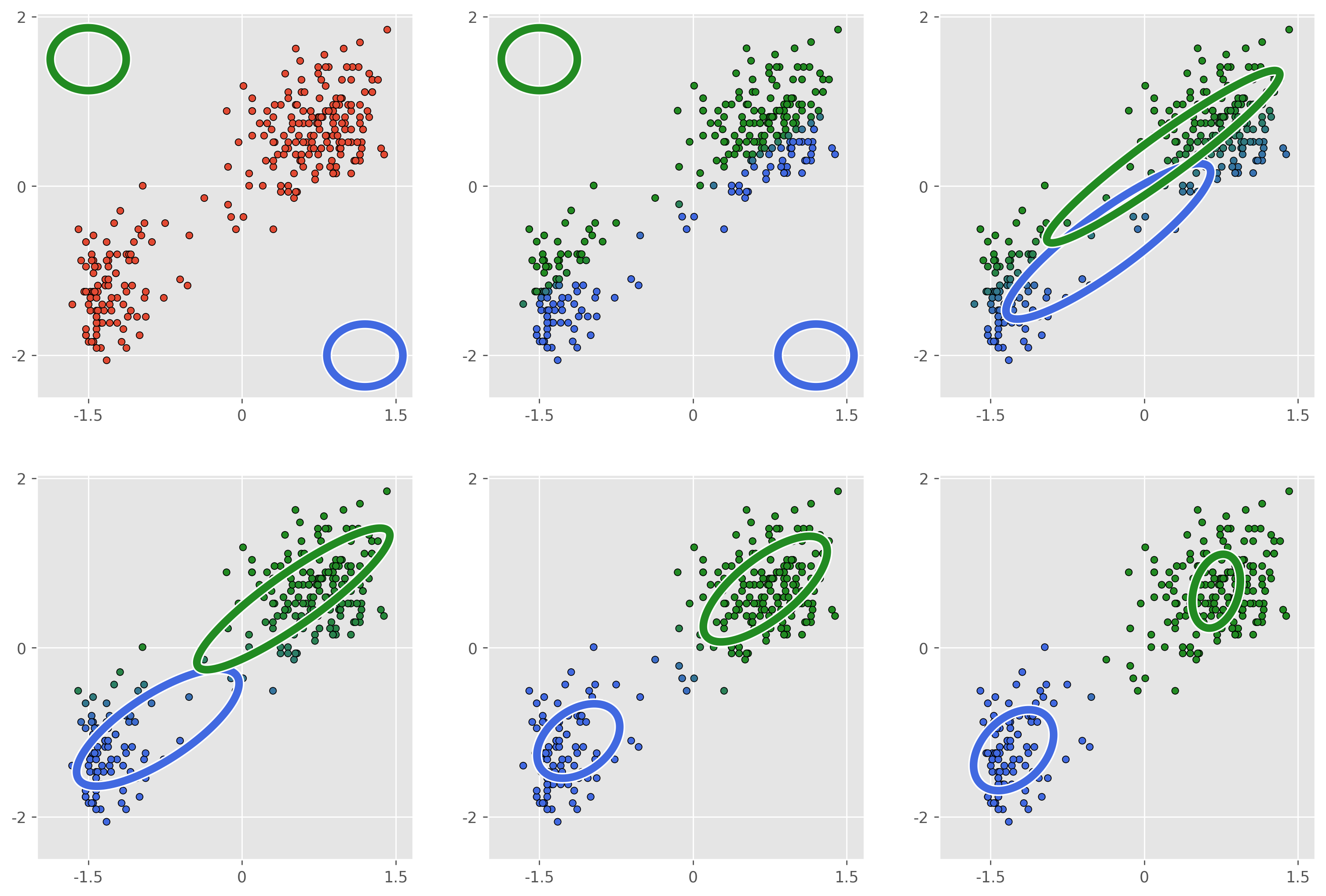
The GMM helps to solve many of the problems we faced with $K$-means. Being a probabalistic model means that we gain access to methods for cross validating our choice of $K$. Unlike $K$-means, increasing our number of clusters will not allow us to artbitrarily increase our log-likelihood. We also gain flexibility in the shape that our clusters can take, though we are still limited to Gaussian ellipsoids. And finally we can quantify our uncertainty for outlier data points which don’t fall cleanly into any one cluster. In terms of initialization, this is still a shortcoming of the GMM as there aren’t many principled ways to ensure good results. In practice we usually run $K$-means++ first, and use this as our cluster initializations for the GMM and this usually works well.

Beyond being two of the most popular clustering techniques, I chose to write about $K$-means and GMMs because they are often used to introduce the Expectation Maximization (EM) algorithm. I didn’t explicitly mention the EM algorithm in this post but briefly it is an algorithm which allows us to perform MLE with latent variable models. I hope to cover the EM algorithm in a future post when my understanding of it is better, and when I do I will link it here.

Appendix

A1
$K$-means implementation

def fit(X, K=2):

    def J(assignments, mu):
        j = 0
        for k in range(K):
            j += (np.linalg.norm(X[assignments == k] - mu[k], axis=1) ** 2).sum()
        return j
    
    def assign_clusters(mu):
        distances = np.zeros(shape=(K, len(X)))
        for k in range(K):
            distances[k] = np.linalg.norm(X - mu[k], axis=1)
        return distances.argmin(axis=0)
    
    def update_mu(assignments, mu):
        new_mu = np.zeros_like(mu)
        for k in range(K):
            new_mu[k] = X[assignments == k].mean()
        return new_mu
    
    mu_updates = []
    assignment_updates = []
    j_scores = []
    
    old_mu = np.array([[1.0, -1.5],
                       [-1.0, 1.5]])
    old_assignments = assign_clusters(old_mu)
    old_j = np.inf
    
    mu_updates.append(old_mu)
    assignment_updates.append(old_assignments)
    j_scores.append(J(old_assignments, old_mu))

    while True:

        new_mu = update_mu(old_assignments, old_mu)
        j_scores.append(J(old_assignments, new_mu))

        new_assignments = assign_clusters(new_mu)
        new_j = J(new_assignments, new_mu)
        j_scores.append(new_j)
        
        if abs(new_j - old_j) < 1e-4:
            break
        
        mu_updates.append(new_mu)
        assignment_updates.append(new_assignments)

        old_mu, old_assignments, old_j = new_mu, new_assignments, new_j
    
    return mu_updates, assignment_updates, j_scores

A2
Chain rule application in GMM derivation $\frac{d}{dx}\log(g(x)) = \frac{g^\prime(x)}{g(x)}$

A3
Derivative of a multivariate normal distribution with respect to $\boldsymbol{\mu}$

A4
GMM implementation

from scipy.stats import multivariate_normal
outer = np.outer
def fit_gmm(X, K=2):

    def compute_LL():
        log_probs = np.zeros((len(X), K))
        for k in range(K):
            log_probs[:, k] += multivariate_normal(mu[:, k], sigma[..., k]).pdf(X) * pi[k]
        log_probs = np.log(log_probs.sum(1))
        return log_probs.sum()
    
    def compute_gamma():
        gamma = np.zeros((len(X), K))
        for k in range(K):
            gamma[:, k] = multivariate_normal(mu[:, k], sigma[..., k]).pdf(X) * pi[k]
        gamma /= gamma.sum(axis=1, keepdims=True)
        return gamma

    def compute_Nk():
        return np.sum(gamma, axis=0)

    def compute_mu():
        mu = np.zeros((2, K))
        for k in range(K):
            mu[:, k] = (gamma[:, k, np.newaxis] * X).sum(axis=0) / N_k[k]
        return mu

    
    def compute_sigma():
        sigma = np.zeros((2, 2, K))
        for k in range(K):
            for n in range(len(X)):
                sigma[..., k] += (gamma[n, k] * outer(X[n] - mu[:, k], X[n] - mu[:, k])) / N_k[k]
        return sigma

    def compute_pi():
        return N_k / len(X)
    
    
    LLs, mus, sigmas, pis, gammas = [], [], [], [], []
    mu = np.array([[1.2, -1.5],
                   [-2.0, 1.5]])
    sigma = np.zeros((2, 2, 2))
    sigma[..., 0] = np.eye(2) * 0.1
    sigma[..., 1] = np.eye(2) * 0.1
    pi = np.array([0.5, 0.5])
    
    mus.append(mu)
    sigmas.append(sigma)
    pis.append(pi)
    
    LL_old = -np.inf
    
    while True:
        gamma = compute_gamma()
        N_k = compute_Nk()
        mu = compute_mu()
        sigma = compute_sigma()
        pi = compute_pi()
        LL_new = compute_LL()

        mus.append(mu)
        sigmas.append(sigma)
        pis.append(pi)
        gammas.append(gamma)
        LLs.append(LL_new)
        if LL_new - LL_old < 1e-9:
            gammas.append(compute_gamma())
            break
        else:
            LL_old = LL_new

    return mus, sigmas, pis, gammas, LLs