Linear Regression
Here I go over the motivations, properties, and interpretations of linear regression
Linear regression is often the first technique taught to undergraduates in a machine learning course. This is a testament to its simplicity, historical significance, and the intuition it provides for designing statistical models. The shortcomings of linear regression also help to motivate the more sophisticated methods that are taught later. In this post I discuss the motivations, properties, and interpretations of linear regression, starting first with simple linear regression.
Predicting House Prices
Suppose we are given a dataset containing the sale price and square footage of a large collection of previously sold homes, and we are tasked with modeling the relationship between these two variables. That is we’d like to be able to reasonably well guess a homes sale price as a function of its square footage.
| Sale Price | Area |
|---|---|
| 221900 | 1180 |
| 180000 | 770 |
| 604000 | 1960 |
| … | … |
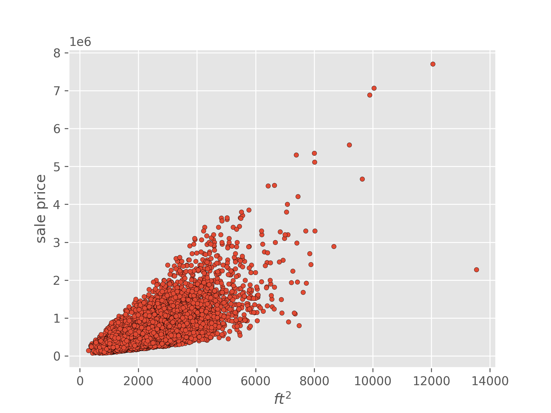
Where would you start? Beyond just predicting the average sale price, the simplest model would be to assume that the two variables are proportional. More specifically, we assume there is some scalar weight which describes how much the sale price is expected to increase for every additional square foot of area.
If the model above was perfectly accurate, the homes in our dataset would fall on a straight line passing through the origin with slope . Of course in reality our data does not lie on a straight line, and the above quantitites are not equal. However, we can fix our equation by adding the house specific sale price not explained by our model . For succinctness I’ll transition to using to denote sale price, to denote area, and to denote the data point.
One obvious pitfall of this model is that our line is constrained to pass through the origin. It may be true that a home with 0 area is worth 0 dollars, but perhaps our dataset doesn’t contain any home prices or square footage below a certain point, or perhaps we just want more flexibility. We can remove this constraint by adding an additive factor to our model.
How then should we go about choosing and , the parameters of our model? Intuitively, the more accurate our model the smaller our errors should be. We could use the sum of the absolute errors (SAE) , but in practice we usually use the sum of the squared errors (SSE) instead.
The reasons why the SSE is often preferred are non-trivial and beyond the scope of this post, but at least one of them will come up in my next one.
Okay so we now have our optimization objective:
In words, we want to choose the and that minimizes the sum of the squared difference between our data and our prediction. To find the forms for the optimal values we can start by taking the partial derivatives of the SSE with respect to each of our parameters A1
As per usual we can set each derivative equal to zero and solve for the parameter.
Finding
Where the bar denotes the average of the variable. Now let’s plug our value for into , set it equal to and solve.
Finding
This form for is completely valid and we could stop here. However, with some rearrangement we can get into a more familiar form. Let’s tackle the numerator first. And now the denominator…
Now we can rewrite
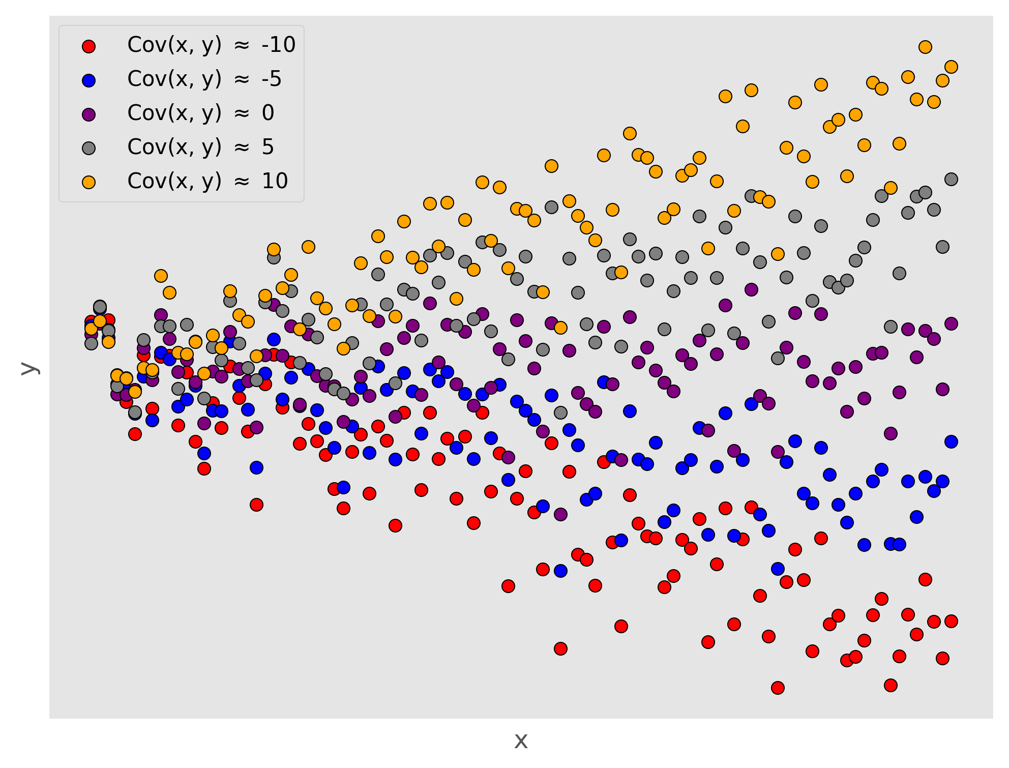
In this form, we can now clearly see that our parameter estimate for is the covariance between our independent and dependent variables scaled by the variance of our independent variable.
If you aren’t familiar, the variance of a random variable is defined as the average squared distance from that random variables mean . It is a measure of the spread of that variable, how much it varies. The covariance is a measure of the joint variability between two random variables. That is, it measures the degree to which two variables change together. The covariance has the following form. Let’s zoom in on the covariance formula, starting with just a single element of the sum. If were to be below its mean and were to be below its mean, the negative signs would cancel and the term would have a positive contribution to the covariance. If instead, were below its mean and was above its mean, that term would have a negative contribution to the covariance. The covariance as a whole measures the average of these contributions and so if small values of tend to co-occur with larger values of and vice versa, the covariance will be negative, indicating a negative linear relationship between the two variables.
How does this inform our interpretation of ? Recall that parameterizes the slope of our linear model, that is how much changes for every unit of . Thus the covariance between and determines whether this change varies downward or upward (the sign of the slope), and the variance of determines over what range this relationship plays out.
where denotes the weight assigned to that particular feature and is the unobserved contributions to the price that aren’t captured by our features, such as market randomness. We include to ensure that the left-hand side and right-hand side are equal, and we refer to as “errors”. Importantly we think of the the weights in the model above as describing some actual, ground-truth process from which we obtain noisy observations (our data). Our goal then is to use those observations to find an approximation of which we denote , that closely matches the true weights. This process is called fitting. To start, let’s rewrite our model using mathematical notation. In doing so we will sacrifice specificity for generality, and succinctness, as well as gain access to a toolbox of mathematical techniques.
First, we will simplify our model and only use one feature, the area (in square feet). Lets denote the area and sale price of the home in our dataset as and respectively. Our model then, looks like
Here is the slope of our line or how much the sale price changes for an increase in the area of the home. If we add an offset term you might recognize this as the slope-intercept form of a line from algebra class.
How then can we estimate our model parameters, and ? In truth we don’t know the true relationship In machine learning we conceptualize fitting (and learning more generally) as an optimization problem, and to solve an optimization problem we need some function to optimize. We want a function that measures how good a particular and are at fitting our data. In practice we usually formulate this function as measuring how bad our choice of parameters are and we try to find the parameters which minimize this function (in my last post on maximum likelihood estimation we took the opposite approach and formulated the optimization as a maximization problem). There are many such functions, referred to as loss functions, that we could choose, and they will all yield slightly different results, but for linear regression the most common choice is to use the least squared error (LSE). If we have different data points, the LSE is defined as
In words, the LSE is the sum over our dataset of the squared differences between our models guess at and the actual sale price given a particular choice of and . The LSE can only equal when our estimate of all the sale prices in our dataset are perfectly correct. Our model is linear and so if this were the case, it would mean that our data lies perfectly on a straight line. Obviously this is highly unrealistic, but if our data follows a linear trend, then optimizing the LSE can result in a decent predictive model.
You might be asking yourself, why optimize the squared differences rather than the absolute differences, isn’t that more intuitive? Admittedly, optimizing the absolute differences is a more intuitive approach, however this is actually less common than using the LSE. This is largely for practical reasons. The LSE has a closed-form solution which we will derive shortly, whereas the least absolute differences requires iterative approximation to converge on an answer. In addition, because the LSE grows quadratically, we end up penalizing bad choices of parameters much more harshly with the LSE than if we were to use absolute differences.
Okay with all that setup lets find our parameter values. We are trying to solve the following optimization problems.
As is the case in most optimization problems we will try to find the values for our parameters when the derivative of our function is equal to . Let’s start with finding our coefficient.
Finding
We begin by taking the derivative of the LSE with respect to
Rather than writing our dataset as a table we will write it as pairs of house features and sale prices. We’ll wrap our features into a vector and denote it in bold , and we will denote our sale prices as , where is an indexing variable used to denote the entry in our dataset. You will often hear referred to as a response variable. Using our particular features, one entry in our dataset now looks like this
This is a good way to understand where our data comes from, but for most of the remainder of this article I’ll use a more general formulation.
We will denote the features of our datapont as a vector , our weights as a vector , and our error terms and reponse variables as scalars .
In linear regression we model our response variables as a linear combination of the elements in the corresponding feature vector. For the data point we have
We can more succinctly write this using vector notation A1.
We can write out the model for our whole dataset if we collect our responses and errors into vectors and our features into a matrix.
Each row of is now a different data point and the columns correspond to that data points features. If we have data points
Appendix
A1
Both partial derivatives of the are obtained through applications of the chain rule